Big Data Lambda Architecture

In order to meet the challenges of Big Data, you must rethink data systems from the ground up. You will discover that some of the most basic ways people manage data in traditional systems like the relational database management system (RDBMS) is too complex for Big Data systems. The simpler, alternative approach is a new paradigm for Big Data. In this article based on chapter 1, author Nathan Marz shows you this approach he has dubbed the “lambda architecture.”

This article is based on Big Data, to be published in Fall 2012. This eBook is available through the Manning Early Access Program (MEAP). Download the eBook instantly from manning.com. All print book purchases include free digital formats (PDF, ePub and Kindle). Visit the book’s page for more information based on Big Data. This content is being reproduced here by permission from Manning Publications.

Author: Nathan Marz

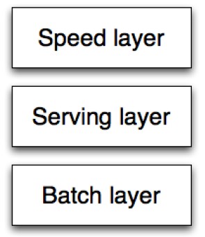
Computing arbitrary functions on an arbitrary dataset in real time is a daunting problem. There is no single tool that provides a complete solution. Instead, you have to use a variety of tools and techniques to build a complete Big Data system. The lambda architecture solves the problem of computing arbitrary functions on arbitrary data in real time by decomposing the problem into three layers: the batch layer, the serving layer, and the speed layer.

Figure 1 – Lambda Architecture

Everything starts from the “query = function(all data)” equation. Ideally, you could literally run your query functions on the fly on a complete dataset to get the results. Unfortunately, even if this were possible, it would take a huge amount of resources to do and would be unreasonably expensive. Imagine having to read a petabyte dataset every time you want to answer the query of someone’s current location.
The alternative approach is to precompute the query function. Let’s call the precomputed query function the batch view. Instead of computing the query on the fly, you read the results from the precomputed view. The precomputed view is indexed so that it can be accessed quickly with random reads. This system looks like this:

Figure 2 – Batch layer

In this system, you run a function on all of the data to get the batch view. Then, when you want to know the value for a query function, you use the precomputed results to complete the query rather than scan through all of the data. The batch view enables you to get the values you need from it very quickly because it’s indexed.

Since this discussion is somewhat abstract, let’s ground it with an example.

Suppose you’re building a web analytics application and you want to query the number of pageviews for a URL on any range of days. If you were computing the query as a function of all the data, you would scan the dataset for pageviews for that URL within that time range and return the count of those results. This, of course, would be enormously expensive because you would have to look at all the pageview data for every query you do.

The batch view approach instead runs a function on all the pageviews to precompute an index from a key of [url, day] to the count of the number of pageviews for that URL for that day. Then, to resolve the query, you retrieve all of the values from that view for all of the days within that time range and sum up the counts to get the result. The precomputed view indexes the data by URL, so you can quickly retrieve all of the data points you need to complete the query.

You might be thinking that there’s something missing from this approach as described so far. Creating the batch view is clearly going to be a high latency operation because it’s running a function on all of the data you have. By the time it finishes, a lot of new data that’s not represented in the batch views will have been collected, and the queries are going to be out of date by many hours. You’re right, but let’s ignore this issue for the moment because we’ll be able to fix it. Let’s pretend that it’s okay for queries to be out of date by a few hours and continue exploring this idea of precomputing a batch view by running a function on the complete dataset.

Batch layer

The portion of the lambda architecture that precomputes the batch views is called the batch layer. The batch layer stores the master copy of the dataset and precomputes batch views on that master dataset. The master dataset can be thought of us a very large list of records.

Figure 3 – Batch layer

The batch layer needs to be able to do two things to do its job: store an immutable, constantly growing master dataset, and compute arbitrary functions on that dataset. The key word here is arbitrary. If you’re going to precompute views on a dataset, you need to be able to do so for any view and any dataset. There’s a class of systems called batch processing systems that are built to do exactly what the batch layer requires. They are very good at storing immutable, constantly growing datasets, and they expose computational primitives to allow you to compute arbitrary functions on those datasets. Hadoop is the canonical example of a batch processing system, and we will use Hadoop to demonstrate the concepts of the batch layer.

Figure 4 – Batch layer

The simplest form of the batch layer can be represented in pseudo-code like this:
function runBatchLayer():
while(true):
recomputeBatchViews()

The batch layer runs in a while(true) loop and continuously recomputes the batch views from scratch. In reality, the batch layer will be a little more involved. This is the best way to think about the batch layer  for the purpose of this article.

The nice thing about the batch layer is that it’s so simple to use. Batch computations are written like single-threaded programs yet automatically parallelize across a cluster of machines. This implicit parallelization makes batch layer computations scale to datasets of any size. It’s easy to write robust, highly scalable computations on the batch layer.

Here’s an example of a batch layer computation. Don’t worry about understanding this code; the point is to show what an inherently parallel program looks like.
Pipe pipe = new Pipe(“counter”);
pipe = new GroupBy(pipe, new Fields(“url”));
pipe = new Every(
pipe,
new Count(new Fields(“count”)),
new Fields(“url”, “count”));
Flow flow = new FlowConnector().connect(
new Hfs(new TextLine(new Fields(“url”)), srcDir),
new StdoutTap(),
pipe);
flow.complete();

This code computes the number of pageviews for every URL, given an input dataset of raw pageviews. What’s interesting about this code is that all of the concurrency challenges of scheduling work, merging results, and dealing with runtime failures (such as machines going down) are done for you. Because the algorithm is written in this way, it can be automatically distributed on a MapReduce cluster, scaling to however many nodes you have available. So, if you have 10 nodes in your MapReduce cluster, the computation will finish about 10 times faster than if you only had one node! At the end of the computation, the output directory will contain a number of files with the results.

Serving layer

The batch layer emits batch views as the result of its functions. The next step is to load the views somewhere so that they can be queried. This is where the serving layer comes in. For example, your batch layer may precompute a batch view containing the pageview count for every [url, hour] pair. That batch view is essentially just a set of flat files though: there’s no way to quickly get the value for a particular URL out of that output.

Figure 5 – Serving layer

The serving layer indexes the batch view and loads it up so it can be efficiently queried to get particular values out of the view. The serving layer is a specialized distributed database that loads in batch views, makes them queryable, and continuously swaps in new versions of a batch view as they’re computed by the batch layer. Since the batch layer usually takes at least a few hours to do an update, the serving layer is updated every few hours.

A serving layer database only requires batch updates and random reads. Most notably, it does not need to support random writes. This is a very important point because random writes cause most of the complexity in databases. By not supporting random writes, serving layer databases can be very simple. That simplicity makes them robust, predictable, easy to configure, and easy to operate. ElephantDB, a serving layer database, is only a few thousand lines of code.

Batch and serving layers satisfy almost all properties

So far you’ve seen how the batch and serving layers can support arbitrary queries on an arbitrary dataset with the tradeoff that queries will be out of date by a few hours. The long update latency is due to the fact that new pieces of data take a few hours to propagate through the batch layer into the serving layer where it can be queried.

The important thing to notice is that, other than low latency updates, the batch and serving layers satisfy every property desired in a Big Data system. Let’s go through them one by one:
* Robust and fault tolerant: The batch layer handles failover when machines go down using replication and restarting computation tasks on other machines. The serving layer uses replication under the hood to ensure availability when servers go down. The batch and serving layers are also human fault tolerant, since, when a mistake is made, you can fix your algorithm or remove the bad data and recompute the views from scratch.
* Scalable—Both the batch layer and serving layers are easily scalable. They can both be implemented as fully distributed systems, whereupon scaling them is as easy as just adding new machines.
* General—The architecture described is as general as it gets. You can compute and update arbitrary views of an arbitrary dataset.
* Extensible—Adding a new view is as easy as adding a new function of the master dataset. Since the master dataset can contain arbitrary data, new types of data can be easily added. If you want to tweak a view, you don’t have to worry about supporting multiple versions of the view in the application. You can simply recompute the entire view from scratch.
* Allows ad hoc queries—The batch layer supports ad-hoc queries innately. All of the data is conveniently available in one location and you’re able to run any function you want on that data.
* Minimal maintenance—The batch and serving layers consist of very few pieces, yet they generalize arbitrarily. So, you only have to maintain a few pieces for a huge number of applications. As explained before, the serving layer databases are simple because they don’t do random writes. Since a serving layer database has so few moving parts, there’s lots less that can go wrong. As a consequence, it’s much less likely that anything will go wrong with a serving layer database, so they are easier to maintain.
* Debuggable—You will always have the inputs and outputs of computations run on the batch layer. In a traditional database, an output can replace the original input—for example, when incrementing a value. In the batch and serving layers, the input is the master dataset and the output is the views. Likewise, you have the inputs and outputs for all of the intermediate steps. Having the inputs and outputs gives you all the information you need to debug when something goes wrong.

The beauty of the batch and serving layers is that they satisfy almost all of the properties you want with a simple and easy to understand approach. There are no concurrency issues to deal with, and it scales trivially. The only property missing is low latency updates. The final layer, the speed layer, fixes this problem.

Speed layer

The serving layer updates whenever the batch layer finishes precomputing a batch view. This means that the only data not represented in the batch views is the data that came in while the precomputation was running. All that’s left to do to have a fully realtime data system—that is, arbitrary functions computed on arbitrary data in real time—is to compensate for those last few hours of data. This is the purpose of the speed layer.

Figure 6 – Speed layer

You can think of the speed layer as similar to the batch layer in that it produces views based on data it receives. There are some key differences, though. One big difference is that, in order to achieve the fastest latencies possible, the speed layer doesn’t look at all the new data at once. Instead, it updates the realtime view as it receives new data instead of recomputing them like the batch layer does. This is called incremental updates as opposed to recomputation updates. Another big difference is that the speed layer only produces views on recent data, whereas the batch layer produces views on the entire dataset.

Let’s continue the example of computing the number of pageviews for a URL over a range of time. The speed layer needs to compensate for pageviews that haven’t been incorporated in the batch views, which will be a few hours of pageviews. Like the batch layer, the speed layer maintains a view from a key [url, hour] to a pageview count. Unlike the batch layer, which recomputes that mapping from scratch each time, the speed layer modifies its view as it receives new data.

When it receives a new pageview, it increments the count for the corresponding [url, hour] in the database.

The speed layer requires databases that support random reads and random writes. Because these databases support random writes, they are orders of magnitude more complex than the databases you use in the serving layer, both in terms of implementation and operation.

The beauty of the lambda architecture is that, once data makes it through the batch layer into the serving layer, the corresponding results in the realtime views. This means you can discard pieces of the are no longer needed realtime view as they’re no longer needed. This is a wonderful result, since the speed layer is way more complex than the batch and serving layers. This property of the lambda architecture is called complexity isolation, meaning that complexity is pushed into a layer whose results are only temporary. If anything ever goes wrong, you can discard the state for entire speed layer and everything will be back to normal within a few hours. This property greatly limits the potential negative impact of the complexity of the speed layer.

The last piece of the lambda architecture is merging the results from the batch and realtime views to quickly compute query functions. For the pageview example, you get the count values for as many of the hours in the range from the batch view as possible. Then, you query the realtime view to get the count values for the remaining hours. You then sum up all the individual counts to get the total number of pageviews over that range. There’s a little work that needs to be done to get the synchronization right between the batch and realtime views. The pattern of merging results from the batch and realtime views is shown in figure 7.

Figure 7 – Satisfying application queries

We’ve covered a lot of material in the past few sections. Let’s do a quick summary of the lambda architecture to nail down how it works.

Summary

The complete lambda architecture is represented in figure 8.

Figure 8 – Lambda architecture diagram

Let’s go through the diagram piece by piece.
* (A)—All new data is sent to both the batch layer and the speed layer. In the batch layer, new data is appended to the master dataset. In the speed layer, the new data is consumed to do incremental updates of the realtime views.
* (B)—The master dataset is an immutable, append-only set of data. The master dataset only contains the rawest information that is not derived from any other information you have.
* (C)—The batch layer precomputes query functions from scratch. The results of the batch layer are called batch views. The batch layer runs in a while(true) loop and continuously recomputes the batch views from scratch. The strength of the batch layer is its ability to compute arbitrary functions on arbitrary data. This gives it the power to support any application.
* (D)—The serving layer indexes the batch views produced by the batch layer and makes it possible to get particular values out of a batch view very quickly. The serving layer is a scalable database that swaps in new batch views as they’re made available. Because of the latency of the batch layer, the results available from the serving layer are always out of date by a few hours.
* (E)—The speed layer compensates for the high latency of updates to the serving layer. It uses fast incremental algorithms and read/write databases to produce realtime views that are always up to date. The speed layer only deals with recent data, because any data older than that has been absorbed into the batch layer and accounted for in the serving layer. The speed layer is significantly more complex than the batch and serving layers, but that complexity is compensated by the fact that the realtime views can be continuously discarded as data makes its way through the batch and serving layers. So, the potential negative impact of that complexity is greatly limited.
* (F)—Queries are resolved by getting results from both the batch and realtime views and merging them together.